pyvplm.addon package
Submodules
pyvplm.addon.comsoladdon module
Specific module to interface variablepowerlaw module with comsol FEM software
- pyvplm.addon.comsoladdon.import_file(file_name: str, parameter_set: pyvplm.core.definition.PositiveParameterSet, units: str)
Function to import .txt file generated by COMSOL (output format). Values can be either expressed within SI units, user defined units or specified units in the parameter name : ‘parameter_name (units)’.
- Parameters
file_name (str) – Name of the saved file with path (example: file_name = ‘./subfolder/name’)
parameter_set (PositiveParameterSet) – Defines the n physical parameters for the studied problem
units (str) – Define what units should be considered for parameters from set * ‘SI’: means parameter is expressed within SI units, no adaptation needed and ‘(units)’ in column name is ignored. * ‘defined’: means parameter is expressed within defined units written in parameter and ‘(units)’ in column name is ignored, adaptation may be performed. * ‘from_file’: means parameter is expressed with file units and adaptation may be performed.
If units are unreadable and from_file option is chosen, it is considered to be expressed in SI units. For parameters not in the defined set, if units are unreadable, there are no units or SI option is chosen, it is considered to be SI otherwise adaptation is performed.
- pyvplm.addon.comsoladdon.save_file(doe_x: numpy.ndarray, file_name: str, parameter_set: pyvplm.core.definition.PositiveParameterSet, is_SI: bool, **kwargs)
Function to save .txt file within COMSOL input format. Values can be either expressed with SI units or user defined units (is_SI, True by default).
- Parameters
doe_x (DOE of the parameter_set either in defined_units or SI units)
file_name (Name of the saved file with path (example: file_name = ‘./subfolder/name’))
parameter_set (Defines the n physical parameters for the studied problem)
is_SI (Define if parameters values are expressed in SI units or units defined by user)
pyvplm.addon.pixdoe module
Addon module generating constrained full-factorial DOE on 2-spaces (pi/x) problems
- pyvplm.addon.pixdoe.apply_constraints(X: numpy.ndarray, Constraints)
Function to test declared constraint and return true vector if an error occurs.
- Parameters
X ([m*n] numpy.ndarray of float or int) – Defines the m DOE points values over the n physical parameters
Constraints (function that should return a [1*m] numpy.ndarray of bool, that validates the m points constraint)
- Returns
Constraints(X) – If dimension mismatch or constraint can’t be applied returns True values (no constraint applied)
- Return type
[1*m] numpy.ndarray of bool
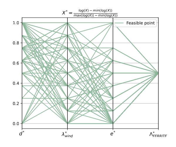
- pyvplm.addon.pixdoe.create_const_doe(parameter_set: pyvplm.core.definition.PositiveParameterSet, pi_set: pyvplm.core.definition.PositiveParameterSet, func_x_to_pi, wished_size: int, **kwargs)
Function to generate a constrained feasible set DOE with repartition on PI not far from nominal fullfact DOE.
- Parameters
parameter_set (Defines the n physical parameters for the studied problem)
pi_set (Defines the k (k<n) dimensionless parameters of the problem (WARNING: no cross-validation with) – parameter_set, uses func_x_to_pi for translation)
func_x_to_pi (Function that translates X physical values into Pi dimensionless values (space transformation matrix))
wished_size (Is the wished size of the final elected X-DOE that represents a constrained fullfact Pi-DOE)
**kwargs (additional argumens) –
level_repartition (numpy.array of int): defines the parameters levels relative repartition,
default is equaly shared (same number of levels) * parameters_constraints (function): returns numpy.array of bool to validate each point in X-DOE, default is [] * pi_constraints (function): returns numpy.array of bool to validate each point in Pi-DOE, default is [] * choice_nb (int): number of returned nearest point from DOE for each nominal DOE point, default is 3 * spacing_division_criteria (int): (>=2) defines the subdivision admitted error in Pi nominal space for feasible point, default is 5 * log_space (bool): defines if fullfact has to be in log space or when false, linear (default is log - True) * track (bool): defines if the different process steps information have to be displayed (default is False) * test_mode (bool): set to False to show plots (default is False)
- Returns
doeXc ([j*n] numpy.array of float) – Represents the elected feasible constrained sets of physical parameters matching spacing criteria with j >= whished_size
doePIc ([j*n] numpy.array of float) – Represents the elected feasible constrained sets of dimensionless parameters matching spacing criteria with j >= whished_size
Example
- define properly the parameter, pi set and transformation function:
>>> In [1]: from pyvplm.core.definition import PositiveParameter, PositiveParameterSet
>>> In [2]: from pyvplm.addon.variablepowerlaw import buckingham_theorem, declare_func_x_to_pi,
reduce_parameter_set
>>> In [3]: u = PositiveParameter('u', [1e-9, 1e-6], 'm', 'Deflection')
>>> In [4]: f = PositiveParameter('f', [150, 500], 'N', 'Load applied')
>>> In [5]: l = PositiveParameter('l', [1, 3], 'm', 'Cantilever length')
>>> In [6]: e = PositiveParameter('e', [60e9, 80e9], 'Pa', 'Young Modulus')
>>> In [7]: d = PositiveParameter('d', [10, 60], 'mm', 'Diameter of cross-section')
>>> In [8]: parameter_set = PositiveParameterSet(u, f, l, e, d)
>>> In [9]: parameter_set.first('u','l')
>>> In [10]: pi_set, _ = buckingham_theorem(parameter_set, False)
>>> In [11]: reduced_parameter_set, reduced_pi_set = reduce_parameter_set(parameter_set, pi_set, 'l')
>>> In [12]: func_x_to_pi = declare_func_x_to_pi(reduced_parameter_set, reduced_pi_set)
- then create a complete DOE:
>>> In [13]: doeXc, doePIc = create_const_doe(reduced_parameter_set, reduced_pi_set, func_x_to_pi, 30,
track=True)

- pyvplm.addon.pixdoe.create_doe(bounds: numpy.ndarray, parameters_level: numpy.ndarray, log_space: bool = True) Tuple[numpy.ndarray, numpy.ndarray]
Functions that generates a fullfact DOE mesh using bounds and levels number.
- Parameters
bounds ([n*2] numpy.ndarray of floats, defines the n parameters [lower, upper] bounds)
parameters_level ([1*n] numpy.ndarray of int, defines the parameters levels)
log_space (Defines if fullfact has to be in log space or when false, linear (default is True))
- Returns
doe_values ([m*n] numpy.ndarray of float) – A fullfact DOE, with n the number of parameters and m the number of experiments (linked to level repartition)
spacing ([1*n] numpy.ndarray) – Represents the DOE’s points spacing on each paramater axis in the space
Example
- define bounds and parameters’ levels:
>>> In [1]: bounds = numpy.array([[10, 100], [100, 1000]], float)
>>> In [2]: parameters_level = numpy.array([2, 3], int)
- generate doe in log space:
>>> In [3]: doe_values, spacing = create_doe(bounds, parameters_level, True)
- returns:
>>> In [4]: doe_values.tolist()
>>> Out[4]: [[10, 100], [100, 100], [10, 316.228], [100, 316.228], [10, 1000], [100, 1000]]
>>> In [5]: spacing.tolist()
>>> Out[5]: [1.0, 0.5]
- pyvplm.addon.pixdoe.declare_does(x_Bounds: numpy.ndarray, x_levels: numpy.ndarray, parameters_constraints, pi_constraints, func_x_to_pi, log_space: bool = True)
Function to generate X and Pi DOE with constraints (called as sub-function script).
- Parameters
x_Bounds ([n*2] numpy.ndarray of floats, defines the n parameters [lower, upper] bounds)
x_levels ([1*n] numpy.ndarray of int, defines the parameters levels)
parameters_constraints, pi_constraints (functions that define parameter and Pi constraints)
func_x_to_pi (function that translates X physical values into Pi dimensionless values) – (space transformation matrix)
log_space (Defines if full-factorial has to be in log space or when false, linear (default is True))
- Returns
doeX ([m*n] numpy.ndarray of float) – A full-factorial DOE, with n the number of parameters and m the number of experiments (linked to level)
doePI ([k*n] numpy.ndarray of float) – Represents the Pi DOE’s points computed from doeX and applying both X and Pi constraints (k<=m)
- pyvplm.addon.pixdoe.elect_nearest(doe: numpy.ndarray, nominal_doe: numpy.ndarray, index: numpy.ndarray)
Function that tries to assign for each point in nominal DOE, one point in feasible DOE elected from its ‘choice_nb’ found indices. The assignments are done point-to-point electing each time the one maximizing minimum relative distance with current elected set. If from available indices they all are already in the set, point is deleted and thus: j<=k (not likely to happen).
- Parameters
doe ([m*n] numpy.ndarray of int or float) – DOE representing m feasible experiments expressed with n parameters with non-optimal spacing
nominal_doe ([k*n] numpy.ndarray of int or float) – Fullfact DOE with k wished experiment (k<<m) expressed with the same n parameters
index ([k*nb_choice] numpy.ndarray of int) – Gathers the corresponding ‘choice_nb’ nearest DOE points indices (computed with :~pixdoe.find_nearest)
- Returns
doe_elected ([j*n] numpy.ndarray of int or float) – Returned DOE with feasible points assigned to reduced nominal DOE (deleted points with no assignment, i.e. all indices already assigned)
reduced_nominal_doe ([j*n] numpy.ndarray of int or float) – Reduced nominal DOE (j<=k), all point are covered with feasible point
Example
to define DOEs and find the nearest points, see
surroundings()- then elect one point for each nominal point:
>>> In [7]: doe_elected, reduced_nominal_doe, max_error = elect_nearest(doe, nominal_doe, index)
>>> In [8]: doe_elected.tolist()
>>> Out[8]: [[100.0, 100.0], [10.0, 251.18864315095797], [100.0, 251.18864315095797], [10.0, 1000.0],
[100.0, 1000.0]]
>>> In [9]: reduced_nominal_doe.tolist()
>>> Out[9]: [[100.0, 100.0], [10.0, 316.22776601683796], [100.0, 316.22776601683796], [10.0, 1000.0],
[100.0, 1000.0]]
>>> In [10]: max_error.tolist()
>>> Out[10]: [0.0, 0.10000000000000009, 0.10000000000000009, 0.0, 0.0]
- pyvplm.addon.pixdoe.find_nearest(doe, nominal_doe, choice_nb, proper_spacing, log_space=True)
Function that returns for each point in nominal DOE point, the indices and max relative error for choice_nb nearest points in feasible DOE. As a distance has to be computed to select nearest in further functions, it is the max value of the relative errors (compared to the bounds) that is returned (this avoids infinite relative error for [0, 0] origin point).
- Parameters
doe ([m*n] numpy.ndarray of int or float) – DOE representing m feasible experiments expressed with n parameters with non-optimal spacing
nominal_doe ([k*n] numpy.ndarray of int or float) – Fullfact DOE with k wished experiment (k<<m) expressed with the same n parameters
choice_nb (int) – Number of the nearest points returned from DOE for each nominal DOE point, criteria is max relative distance error max(x-x_n/(max(x_n)-min(x_n)))
proper_spacing ([n*1] numpy.ndarray of float) – Represents max distance criteria on each DOE axis (i.e. parameter scale)
log_space (bool) – Defines if fullfact has to be in log space or when false, linear (default is True)
- Returns
nearest_index_in_doe – Gathers the corresponding ‘choice_nb’ nearest DOE points indices
- Return type
[k*choice_nb] numpy.ndarray of int
Example
to define DOEs, see
surroundings()- then extract the 2 nearest feasible points for each nominal point:
>>> In [6]: index, max_rel_distance = find_nearest(doe, nominal_doe, 2, proper_spacing, True)
>>> In [7]: index.tolist()
>>> Out[7]: [[0, 4], [3, 7], [8, 12], [11, 15], [20, 16], [23, 19]]
>>> In [8]: max_rel_distance.tolist()
>>> Out[8]: [[0.0, 0.20000000000000018], [0.0, 0.20000000000000018],
[0.10000000000000009, 0.10000000000000009], [0.10000000000000009, 0.10000000000000009]
[0.0, 0.20000000000000018], [0.0, 0.20000000000000018]]
- pyvplm.addon.pixdoe.surroundings(doe, nominal_doe: numpy.ndarray, proper_spacing: numpy.ndarray, LogLin: bool = True) Tuple[numpy.ndarray, numpy.ndarray]
Function to reduce a given nominal DOE on a max distance criteria with points from feasible DOE (‘reachable’ points).
- Parameters
doe ([m*n] numpy.ndarray of int or float) – DOE representing m feasible experiments expressed with n parameters with non-optimal spacing
nominal_doe ([k*n] numpy.ndarray of int or float) – Fullfact DOE with k wished experiment (k<<m) expressed with the same n parameters
proper_spacing ([n*1] numpy.ndarray of float) – Represents max distance criteria on each DOE axis (i.e. parameter scale)
LogLin (defines if fullfact has to be in log space or when false, linear (default is True))
- Returns
reduced_nominal_doe ([l*n] numpy.ndarray) – A reduced set of nominal_doe (l<=k) validating proper_spacing criteria with feasible points from DOE
to_be_removed (numpy.ndarray of bool) – Returns the corresponding indices that do not validate proper_spacing criteria
Example
- define bounds and parameters’ levels:
>>> In [1]: bounds = numpy.array([[10, 100], [100, 1000]], float)
>>> In [2]: parameters_level_nominal = numpy.array([2, 3], int)
>>> In [3]: parameters_level_feasible = numpy.array([4, 6], int)
- generate doe(s) in log space:
>>> In [4]: doe, _ = create_doe(bounds, parameters_level_feasible, True)
>>> In [5]: nominal_doe, proper_spacing = create_doe(bounds, parameters_level_nominal, True)
- search surrounding points:
>>> In [6]: reduced_nominal_doe, to_be_removed = surroundings(doe, nominal_doe, proper_spacing, True)
>>> In [7]: reduced_nominal_doe.tolist()
>>> Out[7]: [[10.0, 100.0], [100.0, 100.0], [10.0, 316.22776601683796], [100.0, 316.22776601683796],
>>>    ...: [10.0, 1000.0], [100.0, 1000.0]]
>>> In [8]: to_be_removed.tolist()
>>> Out[8]: [False, False, False, False, False, False]
pyvplm.addon.variablepowerlaw module
Addon module fitting variable power law response surface on dimensionless parameter computed with FEM
- pyvplm.addon.variablepowerlaw.adapt_parameter_set(parameter_set: pyvplm.core.definition.PositiveParameterSet, pi_set: pyvplm.core.definition.PositiveParameterSet, doe_x: pandas.core.frame.DataFrame, replaced_parameter: str, new_parameter: str, expression: str, description: str) Tuple[pyvplm.core.definition.PositiveParameterSet, pyvplm.core.definition.PositiveParameterSet, pandas.core.frame.DataFrame]
Function that transform physical parameters’ problem (and corresponding DOE) after FEM calculation.
- Parameters
parameter_set (Defines the n physical parameters for the studied problem)
pi_set (Defines the k (k<n) dimensionless parameters of the problem)
doe_x (DOE of the parameter_set in SI units (column names should be of the form ‘parameter_i’))
replaced_parameter (Name of the replaced parameter (should not be a repetitive term, i.e. present in only)
one PI (PI0) term to ensure proper PI spacing)
new_parameter (Name of new parameter (units has to be identical to replaced parameter))
expression (Relation between old and new parameter if x_new = 2*x_old+3*other_parameter,)
write ‘2*x_old+3*other_parameter’
description (Saved description for new parameter)
- Returns
new_parameter_set (Represents the new physical problem)
new_pi_set (Dimensionless parameters set derived from pi_set replacing parameter)
new_doeX (Computed DOE from doeX using expression (relation between parameters))
Example
to define the parameter, pi sets and calculate DOE refer to:
regression_models()- save DOE into dataframe:
>>> In [9]: labels = list(parameter_set.dictionary.keys())
>>> In [10]: doe_x = pandas.DataFrame(doe_x, columns=labels)
- then imagine you want to replace one parameter (after FEM simulation):
>>> In [11]: (new_parameter_set, new_pi_set, new_doeX)
>>>     ...: = adapt_parameter_set(parameter_set, pi_set, doe_x, 'd', 'd_out', 'd+2*e', 'outer diameter')
you are able to perform new regression calculation!
- pyvplm.addon.variablepowerlaw.automatic_buckingham(parameter_set: pyvplm.core.definition.PositiveParameterSet, track: bool = False) Tuple[Any, Dict[str, Any]]
Function that returns all possible pi_set (with lower exponent) from a set of physical parameters. Based on buckingham_theorem function call.
- Parameters
parameter_set (Defines the n physical parameters for the studied problem)
track (Activates information display (default is False))
- Returns
combinatory_pi_set (dict of [1*2] tuples) – Stores pi_set at [0] tuple index and Pi expression (str) list at [1] tuple index
alternative_set_dict (dict of str) – Stores the alternate expressions for widgets display
Example
define a positive set first, see:
write_dimensional_matrix()- search corresponding pi_set:
>>> In [7]: combinatory_pi_set = automatic_buckingham(parameter_set, True)
    [AUTO. BUCKINGHAM] Testing repetitive set 1/120: total alternative pi set size is 1
    [AUTO. BUCKINGHAM] Testing repetitive set 2/120: total alternative pi set size is 1
    [AUTO. BUCKINGHAM] Testing repetitive set 3/120: total alternative pi set size is 1
    ...
>>> In [8]: print(combinatory_pi_set[1][0])
    pi1: pi1 in [1000000.0,2999999999.9999995], l**1.0*u**-1.0
    pi2: pi2 in [1.2e-10,0.0005333333333333334], e**1.0*f**-1.0*u**2.0
    pi3: pi3 in [10000.0,59999999.99999999], d**1.0*u**-1.0
- pyvplm.addon.variablepowerlaw.buckingham_theorem(parameter_set: pyvplm.core.definition.PositiveParameterSet, track: bool = False) Tuple[pyvplm.core.definition.PositiveParameterSet, List[str]]
Function that returns pi_set dimensionless parameters from a set of physical parameters. The Pi expression is lower integer exponent i.e. Pi1 = x1**2*x2**-1 and not x1**1*x2**-0.5 or x1**4*x2**-2
- Parameters
parameter_set (Defines the n physical parameters for the studied problem)
track (Activates information display (default is False))
- Returns
pi_set (PositiveParameterSet) – Defines the k (k<n) dimensionless parameters of the problem
pi_list ([1*k] list of str) – The dimensionless parameters’ expression
Example
define a positive set first, see:
write_dimensional_matrix()- orient repetitive set (using if possible d and l):
>>> In [8]: parameter_set.first('d', 'l')
- search corresponding pi_set:
>>> In [9]: (pi_set, pi_list) = buckingham_theorem(parameter_set, True)
>>> In [10]: print(pi_set)
    Chosen repetitive set is: {d, l}
    pi1: pi1 in [1.666666666666667e-08,9.999999999999999e-05], d**-1.0*u**1.0
    pi2: pi2 in [16.666666666666668,300.0], d**-1.0*l**1.0
    pi3: pi3 in [12000.0,1920000.0000000002], d**2.0*e**1.0*f**-1.0
Note
Repetitive parameters are elected as first pivot point in the order of arrival in parameter set dictionary keys, therefore user can orient repetitive set applying the ‘first’ method on the parameter set (see example)
- pyvplm.addon.variablepowerlaw.compute_echelon_form(in_matrix: numpy.ndarray)
Function that computes a matrix into its echelon form.
- Parameters
in_matrix ([m*n] numpy.ndarray of float or int)
- Returns
out_matrix ([m*n] matrix with echelon form derived from in_matrix)
pivot_matrix ([m*m] pivot matrix to link out_matrix to in_matrix)
pivot_points ([1*k] index of pivot points k = rank(in_matrix)<= min(m, n))
Example
- define dimensional matrix:
>>> In [1]: in_matrix = numpy.array([[0, 1, 0], [1, 1, -2], [0, 1, 0], [1, -1, -2], [0, 1, 0]], int)
- perform echelon function:
>>> In [2]: (out_matrix, pivot_matrix, pivot_points) = compute_echelon_form(in_matrix)
>>> In [3]: nc = len(out_matrix[0]
>>> In [4]: nr = len(out_matrix)
>>> In [5]: print([[float(out_matrix[ir][ic]) for ic in range(nc)] for ir in range(nr)])
    [[1.0, 0.0, -2.0], [0.0, 1.0, 0.0], [0.0, 0.0, 0.0], [0.0, 0.0, 0.0], [0.0, 0.0, 0.0]]
>>> In [6]: print([[float(pivot[nr][nc]) for nc in range(len(pivot[0]))] for nr in range(len(pivot))])
    [[-1.0, 1.0, 0.0, 0.0, 0.0], [1.0, 0.0, 0.0, 0.0, 0.0], [-1.0, 0.0, 1.0, 0.0, 0.0],
    [2.0, -1.0, 0.0, 1.0, 0.0], [-1.0, 0.0, 0.0, 0.0, 1.0]]
>>> In [7]: print(pivot_points)
    [1, 0]
- pyvplm.addon.variablepowerlaw.concatenate_expression(expression: str, pi_list: List[str]) str
Function that transform regression model expression into latex form with concatenation (only for power-laws).
- Parameters
expression (Expression of the regression model)
pi_list (Defines the pi expressions (default is pi1, pi2…))
- Returns
new_expression
- Return type
Represents the new model formula in latex form
Example
- define expression and list:
>>> In [1]: expression = 'log(pi1) = 2.33011+1.35000*log(pi2)-0.25004*log(pi3)+0.04200*log(pi2)*log(pi3)+'
>>>    ...: '0.17000*log(pi2)**2'
>>> In [2]: pi_list = ['\pi_{1}','\pi_{2}','\pi_{3}']
- adapt expression:
concatenate_expression(expression, pi_list)
- pyvplm.addon.variablepowerlaw.declare_constraints(parameters_set: pyvplm.core.definition.PositiveParameterSet, constraint_set: pyvplm.core.definition.ConstraintSet)
Functions that declare constraint=f(X_doe)/f(PI_doe) to return validity of a DoE set .
- Parameters
parameters_set (Defines the n physical/dimensionless parameters (be careful to share set)
with pixdoe.create_const_doe)
constraint_set (Defines the constraints that apply on the parameters from parameters_set)
- Returns
f – a function of X, X being a [m*k] (k<=n) numpy.ndarray of float representing parameters values which returns a [m*1] numpy.ndarray of bool corresponding to the DoE validity
- Return type
function
- pyvplm.addon.variablepowerlaw.declare_func_x_to_pi(parameters_set: pyvplm.core.definition.PositiveParameterSet, pi_set: pyvplm.core.definition.PositiveParameterSet)
Functions that declare pi=f(x) to transform parameters set values into pi set values.
- Parameters
parameters_set (Defines the n physical parameters for the studied problem)
pi_set (Defines the k (k<n) dimensionless parameters of the problem)
- Returns
f – a function of x, x being a [m*n] numpy.ndarray of float representing physical parameters values which returns a [m*k] numpy.ndarray of float corresponding to the dimensionless parameters values
- Return type
function
Example
define a positive set first, see:
write_dimensional_matrix()- define pi set using buckingham:
>>> In [7]: pi_set, _ = buckingham_theorem(parameter_set, False)
- set x values:
>>> In [8]: x = [[1, 1.5, 2, 3, 5],[0.1, 2, 1, 2, 1],[2, 1, 3, 1.5, 2]]
- declare function and compute y values:
>>> In [9]: func_x_to_pi = declare_func_x_to_pi(parameter_set, pi_set)
>>> In [10]: func_x_to_pi(x)
    array([[ 2.  ,  2.  ,  5.  ],
           [10.  ,  0.01, 10.  ],
           [ 1.5 ,  6.  ,  1.  ]])
- pyvplm.addon.variablepowerlaw.force_buckingham(parameter_set: pyvplm.core.definition.PositiveParameterSet, *pi_list: Union[Iterable, Tuple[str]]) pyvplm.core.definition.PositiveParameterSet
Function used to define manually a dimensionless set of parameters. Parameters availability, pi expression and dimension or even pi matrix rank are checked.
- Parameters
parameter_set (Defines the n physical parameters for the studied problem)
*pi_list (Defines the Pi dimensionless parameters’ expression of the problem)
- Returns
pi_set – Defines the k (k<n) dimensionless parameters of the problem
- Return type
Example
define a positive set first, see:
write_dimensional_matrix()- force pi set:
>>> In [7]: pi_set = force_buckingham(parameter_set, 'l/u', 'e/f*u^2', 'd/u')
>>> In [8]: print(pi_set)
    pi1: pi1 in [1000000.0,2999999999.9999995], u**-1.0*l**1.0
    pi2: pi2 in [1.2e-10,0.0005333333333333334], u**2.0*f**-1.0*e**1.0
    pi3: pi3 in [10000.0,59999999.99999999], u**-1.0*d**1.0
Note
The analysis is conducted on Pi dimension, rank of Pi-parameter exponents, global expression and number of Pi compared to dimensional matrix rank and parameters number. The ‘understood expression’ is visible by printing pi_set.
- pyvplm.addon.variablepowerlaw.import_csv(file_name: str, parameter_set: pyvplm.core.definition.PositiveParameterSet)
Function to import .CSV with column label syntax as ‘param_name’ or ‘param_name [units]’. Auto-adaptation to SI-units is performed and parameters out of set are ignored/deleted.
- Parameters
file_name (Name of the saved file with path (example: file_name = ‘./subfolder/name’))
parameter_set (Defines the n physical parameters for the studied problem)
- pyvplm.addon.variablepowerlaw.latex_pi_expression(pi_set: pyvplm.core.definition.PositiveParameterSet, parameter_set: pyvplm.core.definition.PositiveParameterSet)
Function to write pi description in latex form: *internal* to
pi_sensitivity()andpi_dependency()
- pyvplm.addon.variablepowerlaw.perform_regression(doe_pi: numpy.ndarray, models, chosen_model, **kwargs)
Function to perform regresion using models expression form (with replaced coefficients).
- Parameters
doe_pi (numpy.ndarray) – DOE of the pi_set
models (specific) – Output of
variablepowerlaw().chosen_model (int) – The elected regression model number
**kwargs (additional argumens) –
pi_list (list of str): the name/expression of pi (default is pi1, pi2, pi3…)
latex (bool): define if graph legend font should be latex (default is False) - may cause some
issues if used * removed_pi (list): list of indexes of removed pi numbers * max_pi_nb (int): maximum potential pi number that could appear in any expression (only useful if some pi mubers have been removed) * eff_pi_0 (int): effective pi0 index in pi_list (used only if some pi numbers have been removed) * no_plots (bool): for GUI use, will return Y and Yreg as well as expression and latex_expression, will not plot anything
Example
to define regression models refer to:
regression_models()- then perform regression on model n°8 to show detailed results on model fit and error:
>>> In[24]: perform_regression(doe_pi, models, chosen_model=8)

- pyvplm.addon.variablepowerlaw.pi_dependency(pi_set: pyvplm.core.definition.PositiveParameterSet, doe_pi: numpy.ndarray, useWidgets: bool, **kwargs)
Function to perform dependency analysis on dimensionless parameters.
- Parameters
pi_set (Set of dimensionless parameters)
doe_pi (DOE of the complete pi_set (except pi0))
useWidgets (Boolean to choose if widgets displayed (set to True within Jupyther Notebook))
**kwargs (additional argumens) –
x_list (list of str): name of the different pi to be defined as x-axis (default: all)
y_list (list of str): name of the different pi to be defined as y-axis (default: all)
order (int): the order chosen for power-law or polynomial regression model (default is 2)
threshold (float): in ]0,1[ the lower limit to consider regression for plot (default is 0.9)
figwidth (int): change figure width (default is 16 in widgets mode)
xlabel_size (int): set x-axis label font size (default is 16)
Example
to load a doe example: see
pi_sensitivity()- then perform dependency analysis:
>>> In [11]: pi_dependency(pi_set, doe_pi, useWidgets=False)

- pyvplm.addon.variablepowerlaw.pi_dependency_sub(pi_set: pyvplm.core.definition.PositiveParameterSet, doe_pi: numpy.ndarray, **kwargs)
Sub-function of
pi_dependency()
- pyvplm.addon.variablepowerlaw.pi_sensitivity(pi_set: pyvplm.core.definition.PositiveParameterSet, doe_pi: numpy.ndarray, use_widgets: bool, **kwargs)
Function to perform sensitivity analysis on dimensionless parameters according to specific performance.
- Parameters
pi_set (Set of dimensionless parameters)
doe_pi (DOE of the complete pi_set (except pi0))
use_widgets (Boolean to choose if widgets displayed (set to True within Jupyther Notebook))
**kwargs (additional argumens) –
pi0 (list of str): name of the different pi0 = f(pi…) considered as design drivers
piN (list of str): name of the f(pi1, pi2, …, piN) considered as secondary parameters
latex (bool): display in latex format
figwidth (int): change figure width (default is 16 in widgets mode)
zero_ymin (bool): set y-axis minimum value to 0 (default is False)
xlabel_size (int): set x-axis label font size (default is 18)
Example
- to load a doe example:
>>> In [1]: doe_pi = pandas.read_excel('./pi_analysis_example.xls')
>>> In [2]: doe_pi = doe[['pj','pfe','pi2','pi3','pi4','pi5','pi6']].values
>>> In [3]: pi1 = PositiveParameter('pi1',[0.1,1],'','p_j')
>>> In [4]: pi2 = PositiveParameter('pi2',[0.1,1],'','p_fe')
>>> In [5]: pi3 = PositiveParameter('pi3',[0.1,1],'','d_i*d_e**-1')
>>> In [6]: pi4 = PositiveParameter('pi4',[0.1,1],'','e_tooth*d_e**-1*n')
>>> In [7]: pi5 = PositiveParameter('pi5',[0.1,1],'','e_yoke*d_e**-1*n')
>>> In [8]: pi6 = PositiveParameter('pi6',[0.1,1],'','w_pm*d_e**-1')
>>> In [9]: pi7 = PositiveParameter('pi7',[0.1,1],'','r_i*d_e**-1')
>>> In [10]: pi_set = PositiveParameterSet(pi1, pi2, pi3, pi4, pi5, pi6, pi7)
- then perform sensitivity analysis:
>>> In [11]: pi_sensitivity(pi_set, doe_pi, False, pi0=['pi1', 'pi2'], piN=['pi3', 'pi4', 'pi5', 'pi6',
>>>     ...: 'pi7'])
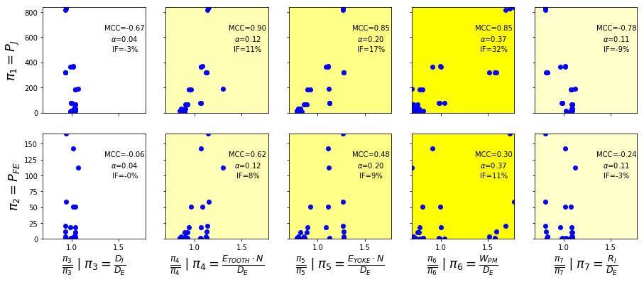
Note
Within Jupyter Notebook, rendering will be slightly different with compressed size in X-axis to be printed within one page width and labels adapted consequently. The graph indices are:
MCC: Maximum Correlation Coefficient is the maximum value between Spearman and Pearson coefficients
alpha: variability coefficient is the ratio between parameter standard deviation and average value
IF: Impact Factor is the product of both previous coefficients
- pyvplm.addon.variablepowerlaw.pi_sensitivity_sub(pi_set: pyvplm.core.definition.PositiveParameterSet, doe_pi: numpy.ndarray, **kwargs)
Sub-function of
pi_sensitivity()
- pyvplm.addon.variablepowerlaw.reduce_parameter_set(parameter_set: pyvplm.core.definition.PositiveParameterSet, pi_set: pyvplm.core.definition.PositiveParameterSet, elected_output: str) Tuple[pyvplm.core.definition.PositiveParameterSet, pyvplm.core.definition.PositiveParameterSet]
Function that reduces physical parameters and Pi set extracting output physical parameter and Pi0.
- Parameters
parameter_set (Defines the n physical parameters for the studied problem)
pi_set (Defines the k (k<n) dimensionless parameters of the problem)
elected_output (Parameter that represents FEM output)
- Returns
reduced_parameter_set (Parameter set reduced by elected_output)
reduced_pi_set (Pi set reduced by Pi0 (dimensionless parameter countaining output parameter))
Example
to define the parameter and pi sets refer to:
buckingham_theorem()- reduce sets considering ‘u’ is the output:
>>> In [9]: reduced_parameter_set, reduced_pi_set = reduce_parameter_set(parameter_set, pi_set, 'u')
- then declare transformation function and create DOE:
>>> In [10]: func_x_to_pi = declare_func_x_to_pi(reduced_parameter_set, reduced_pi_set)
>>> In [11]: from pyvplm.addon.pixdoe import create_const_doe
>>> In [12]: doeX, _ = create_const_doe(reduced_parameter_set, reduced_pi_set, func_x_to_pi, 50)
>>> In [13]: doeX = pandas.DataFrame(doeX, columns=list(reduced_parameter_set.dictionary.keys()))
- pyvplm.addon.variablepowerlaw.regression_models(doe: numpy.ndarray, elected_pi0: str, order: int, **kwargs) Union[Tuple[Dict, Any, Any], Dict]
Functions that calculate the regression model coefficient with increasing model complexity. The added terms for complexity increase are sorted depending on their regression coefficient value on standardized pi. For more information on regression see Scipy linalg method
lstsq()- Parameters
doe ([m*k] numpy.ndarray of float or int) – Represents the elected feasible constrained sets of m experiments values expressed over the k dimensionless parameters
elected_pi0 (Selected pi for regression: syntax is ‘pin’ with n>=1 and n<=k)
order (Model order >=1) –
- Order 2 in log_space=True is :
log(pi0) = log(cst) + a1*log(pi1) + a11*log(pi1)**2 + a12*log(pi1)*log(pi2) + a2*log(pi2) + a22*log(pi2)**2
- Order 2 in log_space=False is :
pi0 = cst + a1*pi1 + a11*pi1**2 + a12*pi1*pi2 + a2*pi2 + a22*pi2
**kwargs (additional argumens) –
ymax_axis (float): set y-axis maximum value representing relative error, 100=100%
(default value) * log_space (bool): define if polynomial regression should be performed within logarithmic space (True) or linear (False) * latex (bool): define if graph legend font should be latex (default is False) - may cause some issues if used * plots (bool): overrules test_mode and allows showing plots * skip_cross_validation (bool): for a big amount of data (data nb > 10 * nb models) you may want to skip cross-validation for time-calculation purpose, in that case only a trained dataset is calculated and error calculation is only performed on trained set (default is False). * force_choice (int): forces the choice of the regression criteria (1 => max(abs(error)), … ) * removed_pi (list): list of indexes of removed pi to be ignored * eff_pi0 (int): effective pi0 index in the modfied DOE (used only with removed_pi) * return_axes (bool): returns the axes objects for the plots if True (default is False) * fig_size (tuple): tuple of 2 numbers specifying the width and height of the plot in inches
- Returns
models –
- Stores the different regression models information as for model ‘i’:
dict[i][0]: str of the model expression
dict[i][1]: numpy.ndarray of the regression coefficients
dict[i][2]: pandas.DataFrame of the trained set (max abs(e), average abs(e),
average e and sigma e) * dict[i][3]: pandas.DataFrame of the tested set (max abs(e), average abs(e), average e and sigma e)
Where e represents the relative error on elected_pi0>0 in %
- Additional data is saved in:
dict[‘max abs(e)’]: (1*2) tuple containing trained and test sets max absolute relative error
dict[‘ave. abs(e)’]: (1*2) tuple containing trained and test sets average absolute relative error
dict[‘ave. e’]: (1*2) tuple containing trained and test sets average relative error
dict[‘sigma e’]: (1*2) tuple containing trained and test sets standard deviation on relative error
- Return type
dict of [1*4] tuple
Example
to define the parameter and pi sets and generate DOE: to define the parameter and pi sets refer to:
reduce_parameter_set()- generate mathematic relation between Pi parameters knowing pi1=l/u and following formulas:
>>> In [14]: PI2 = doeX['e']*(1/doeX['f'])* doeX['u']**2
>>> In [15]: PI3 = doeX['d']*(1/doeX['u'])
>>> In [16]: PI1 = numpy.zeros(len(PI2))
>>> In [17]: for idx in range(len(PI1)):
>>>     ...:        PI1[idx] = (10**2.33)*
>>>     ...:        (PI2[idx]**(1.35+0.17*numpy.log10(PI2[idx])+0.042*numpy.log10(PI3[idx])))*
>>>     ...:        (PI3[idx]**-0.25) + (random.random()-0.5)/1000000
>>> In [18]: l_values = PI1 * doeX['u']
>>> In [19]: doeX['l'] = l_values
>>> In [20]: doeX = doeX[list(parameter_set.dictionary.keys())]
>>> In [21]: func_x_to_pi = declare_func_x_to_pi(parameter_set, pi_set)
>>> In [22]: doePI = func_x_to_pi(doeX.values)
>>> In [23]: models = regression_models(doePI, 'pi1', 3)

- pyvplm.addon.variablepowerlaw.save_csv(doe_x: numpy.ndarray, file_name: str, parameter_set: pyvplm.core.definition.PositiveParameterSet, is_SI: bool)
Function to save .CSV with column label syntax as ‘param_name [units]’. With units either defined by user or SI (is_SI, True by default).
- Parameters
doe_x (DOE of the parameter_set either in defined_units or SI units)
file_name (Name of the saved file with path (example: file_name = ‘./subfolder/name’))
parameter_set (Defines the n physical parameters for the studied problem)
is_SI (Define if parameters values are expressed in SI units or units defined by user)
- pyvplm.addon.variablepowerlaw.write_dimensional_matrix(parameter_set: pyvplm.core.definition.PositiveParameterSet) pandas.core.frame.DataFrame
Function to extract dimensional matrix from a PositiveParameterSet.
- Parameters
parameter_set (defines the n physical parameters for the studied problem)
- Returns
dimensional_matrix
- Return type
column labels refers to the parameters names and rows to the dimensions
Example
- define a positive set first:
>>> In [1]: u = PositiveParameter('u', [1e-9,1e-6], 'm', 'Deflection')
>>> In [2]: f = PositiveParameter('f', [150,500], 'N', 'Load applied')
>>> In [3]: l = PositiveParameter('l', [1,3], 'm', 'Cantilever length')
>>> In [4]: e = PositiveParameter('e', [60e9,80e9], 'Pa', 'Young Modulus')
>>> In [5]: d = PositiveParameter('d', [10,60], 'mm', 'Diameter of cross-section')
>>> In [6]: parameter_set = PositiveParameterSet(u, f, l, e, d)
- then, apply function:
>>> In [7]: dimensional_matrix = write_dimensional_matrix(parameter_set)
>>> In [8]: dimensional_matrix.values
>>> Out[8]: [[1, 0, 0], [1, 1, -2], [1, 0, 0], [-1, 1, -2], [1, 0, 0]]